Climate Modeling: Evidence from Neural Diffusion Equations
This paper introduces a new way to model climate using advanced machine learning techniques that combine neural networks with mathematical equations that describe how things spread, like temperature or air. The new model shows better results than previous methods.
Content & Liability Disclaimer
This article and its accompanying video are automated summaries derived from Climate Modeling with Neural Diffusion Equations by Jeehyun Hwang, Jeongwhan Choi, Hwangyong Choi, Kookjin Lee, Dongeun Lee, Noseong Park. The original research was conducted solely by the paper's authors; PDFdigest did not conduct any of the research and makes no claims of ownership over the underlying scientific work.
The video narration is generated by artificial intelligence and references the paper's authors for attribution. The video is not narrated by any of the paper's authors. This content may contain inaccuracies, omissions, or misinterpretations of the original research. First-person language (e.g., "we found", "our results") reflects the original authors' voice, not PDFdigest's. Always read the original paper for accurate, verified information before making any decisions based on this content.
This content is provided "as is" without any warranties, express or implied. Simulated systems OÜ, its officers, directors, employees, and agents shall not be liable for any direct, indirect, incidental, special, consequential, or punitive damages arising from your use of, reliance on, or access to this content, including but not limited to errors, omissions, or misinterpretations of the original research. This disclaimer applies to the fullest extent permitted by applicable law.
- 1 In the case of climate modeling, an area to model is frequently abstracted by a grid network (or a small-world network) and each grid cell corresponds to an element in h(t) .
- 2 Climatologists study the natural factors that cause climate change, using past information to help predict future climate change.
- 3 De Bezenac et al. used transport physics (diffusion and advection) to predict the sea surface temperature, but this is limited to a regular grid.
- 4 Due to the uncertain nature of real-world climate data, however, our problem definition is to model the relationships among various noisy climate factors.
Introduction
Deep learning-based climate modeling (or weather forecasting) is an emerging topic and a brand-new application area – . Owing to the recent advancement of the differential equation-inspired deep learning – , this specific topic is gathering much attention from the research community.
In NODEs, more specifically, we solve an integral problem of h(t 1 ) = h(t 0 ) + t1 t0 f (h(t), t; θ f )dt, where h is a vector that contains a set of values that change over time t ∈ [0, T ] and f (h(t), t; θ f ) = dh.
In other words, the multi-dimensional vector h(t 1 ) at time t 1 > t 0 is calculated by adding the sum of the changes in [t 0 , t 1 ] to h(t 0 ).
3) NOAA Data: For this dataset which does not have edge features, DPGN, GN-only and GN-skip cannot be tested because they require edge features.
Methodology
The seminal paper, titled neural ordinary differential equations (NODEs), discovered that residual networks are equivalent to the explicit Euler method to solve ODE problems . We typically use the mean squared error (MSE) as a loss function since climate modeling or weather forecasting is a regression problem.
Study Design
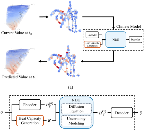
Whereas various recurrent neural network models and regression models can be used for this purpose, we propose to use the diffusion equation under the regime of NODEs to model the physical dynamics governing the spread of temperature, air, etc.
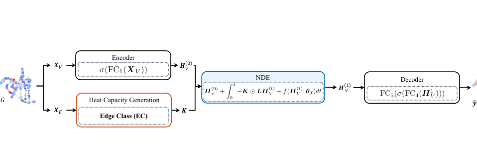
The overall workflow of our method is shown in Fig. 1 .
Results & Findings
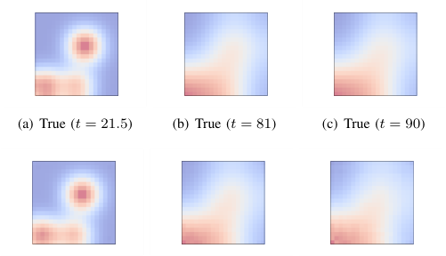
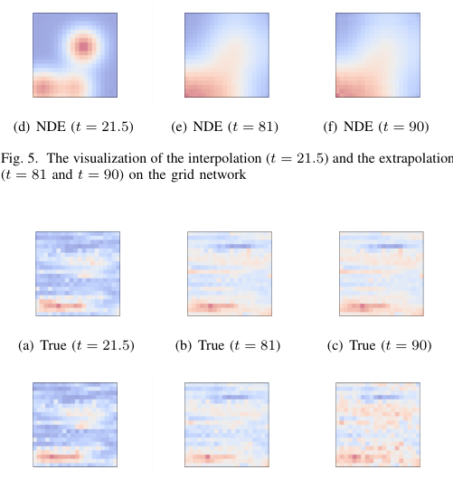
In the case of climate modeling, an area to model is frequently abstracted by a grid network (or a small-world network) and each grid cell corresponds to an element in h(t) . The NDE layer consists of two parts: i) the diffusion equation and ii) the neural networkbased uncertainty model f .
- In the case of climate modeling, an area to model is frequently abstracted by a grid network (or a small-world network) and each grid cell corresponds.
- The NDE layer consists of two parts: i) the diffusion equation and ii) the neural networkbased uncertainty model f .
- To further increase the accuracy, in our case we extend the definition of the time-derivative of h(t) to dh (t) dt = -kLh(t) + f (h(t).
- The synthetic datasets include a grid and small-world network (with and without noises injected into the data) -we note that climate models typically assume either a.
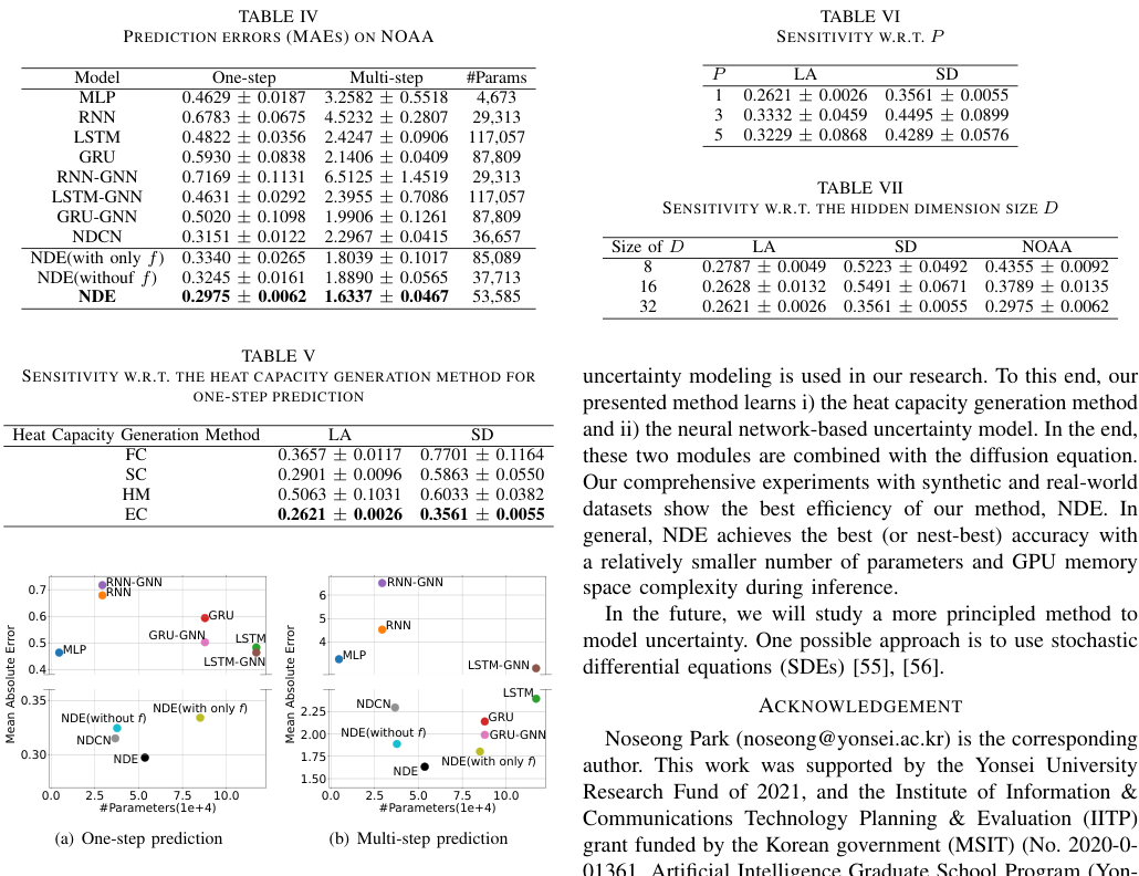
- 1) We design a climate forecasting model with the diffusion equation, the neural network-based uncertainty modeling, and the heat capacity generation methods.
De Bezenac et al. used transport physics (diffusion and advection) to predict the sea surface temperature, but this is limited to a regular grid.
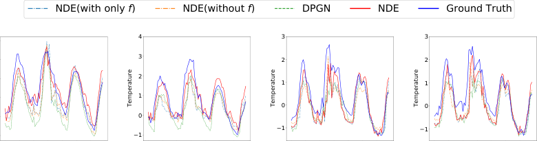
In realworld environments, however, it is hard to say that diffusion processes are completely governed by the diffusion equation -in particular, we observe in our experiments that diffusion processes around large cities have non-trivial uncertainties that cannot be solely described.
How PDFdigest Helps You Understand Research
Instant Paper Analysis
Get structured summaries and key findings from dense PDFs in seconds.
Visual Explanations
Turn complex methods, figures, and results into clearer visual breakdowns.
AI-Powered Q&A
Ask focused questions and get answers grounded in the paper.
Practical Applications
One possible approach is to use stochastic differential equations (SDEs) , .
I. Introduction
The introduction discusses the emergence of deep learning in climate modeling, highlighting the significance of NODEs and their application in solving ordinary differential equations (ODEs) for climate data.
A. Neural Ordinary Differential Equations (NODEs)
NODEs are introduced as a method to solve initial value problems using neural networks to approximate ODE functions, emphasizing their application in climate modeling.
Source Paper Figures and Captions
Frequently Asked Questions
Owing to the recent advancement of the differential equation-inspired deep learning – , this specific topic is gathering much attention from the research community. In other words, the multi-dimensional vector h(t 1 ) at time t 1 > t 0 is calculated.
The seminal paper, titled neural ordinary differential equations (NODEs), discovered that residual networks are equivalent to the explicit Euler method to solve ODE problems . In most cases, weather stations and their sensing values are converted into a graph annotate with node.
In the case of climate modeling, an area to model is frequently abstracted by a grid network (or a small-world network) and each grid cell corresponds to an element in h(t) . Climatologists study the natural factors that cause climate change, using.
Therefore, training residual networks is solving ODE problems specialized in image classification, according to them. Therefore, it is one of the most crucial points in our model to learn a reliable heat capacity.
De Bezenac et al. used transport physics (diffusion and advection) to predict the sea surface temperature, but this is limited to a regular grid. In realworld environments, however, it is hard to say that diffusion processes are completely governed by the diffusion.
This paper introduces a new way to model climate using advanced machine learning techniques that combine neural networks with mathematical equations that describe how things spread, like temperature or air. The new model shows better results than previous methods.