Intrinsic Non-stationary Covariance Function for Climate Modeling
This paper discusses a new way to model climate data, particularly sea level changes, by using a special mathematical function that adapts to different regions and conditions. This approach helps improve predictions about future climate impacts.
Content & Liability Disclaimer
This article and its accompanying video are automated summaries derived from Intrinsic Non-stationary Covariance Function for Climate Modeling by Chintan A Dalal, Vladimir Pavlovic, Robert E Kopp. The original research was conducted solely by the paper's authors; PDFdigest did not conduct any of the research and makes no claims of ownership over the underlying scientific work.
The video narration is generated by artificial intelligence and references the paper's authors for attribution. The video is not narrated by any of the paper's authors. This content may contain inaccuracies, omissions, or misinterpretations of the original research. First-person language (e.g., "we found", "our results") reflects the original authors' voice, not PDFdigest's. Always read the original paper for accurate, verified information before making any decisions based on this content.
This content is provided "as is" without any warranties, express or implied. Simulated systems OÜ, its officers, directors, employees, and agents shall not be liable for any direct, indirect, incidental, special, consequential, or punitive damages arising from your use of, reliance on, or access to this content, including but not limited to errors, omissions, or misinterpretations of the original research. This disclaimer applies to the fullest extent permitted by applicable law.
- 1 To compute the objective function ψ for the space of spatially smooth kernels ({Σ i } N i=1 ), we assume that ψ lies on the Riemannian manifold M of positive definite matrices S + (d, R).
- 2 defined the empirical Riemannian mean Σ ∈ S + (d, R), and gave an iterative form of Σ as a local minimum of the objective function.
- 3 We first obtain initial smooth estimates of the CLS (Σ i ) by Equation ( 3 ), and then we update Σ i with the aim of modeling the intrinsic function ψ ij using our approach proposed in Algorithm 2.
- 4 The standard kriging (GP) model tries to recover the underlying function, f , where y i ∼ f (x i ) + η, from n observed data points {(x, y)} n i=1 .
Introduction
Designing a covariance function that can capture the geospatial random field of natural processes is useful for understanding the changes occurring in climate related variables. For example, ongoing sea level changes provide an important context for understanding future coastal flood risks .
However, most of the climate related datasets at a global scale suffer from statistical issues of non-stationarity and non-uniformly smooth spatial boundaries.
In this paper, we design a covariance function which addresses these issues in the datasets.
Future work will explore the application and methods of our intrinsic covariance function to such geospatial datasets, with the larger goal of aiding in the assessment of future climate related risks.
Research Question
) is an objective function of the form:. To compute the objective function ψ for the space of spatially smooth kernels ({Σ i } N i=1 ), we assume that ψ lies on the Riemannian manifold M of positive definite matrices S + (d, R).
defined the empirical Riemannian mean Σ ∈ S + (d, R), and gave an iterative form of Σ as a local minimum of the objective function.
We first obtain initial smooth estimates of the CLS (Σ i ) by Equation ( 3 ), and then we update Σ i with the aim of modeling the intrinsic function ψ ij using our approach proposed in Algorithm 2.
Methodology
Covariance functions are a key element in the regression of geospatial data (kriging). For standard kriging models (GP), the methods given in are widely used in many climate models, including models of the sea level data, because it gives a non-parametric method for analyzing such a geospatial random field.
Study Design
The approach of setting fixed grids renders this method unviable for datasets with non-uniformly smooth boundaries.
Our method maintains the appropriate smoothness in the latent space of Σ i due to the second-order intrinsic statistics on the Riemannian manifold.
How PDFdigest Helps You Understand Research
Instant Paper Analysis
Get structured summaries and key findings from dense PDFs in seconds.
Visual Explanations
Turn complex methods, figures, and results into clearer visual breakdowns.
AI-Powered Q&A
Ask focused questions and get answers grounded in the paper.
Results & Findings
Addressing this issue, which we call the nonuniformly smooth spatial boundary issue, aids in modeling the non-stationary covariance function by capturing the underlying correlation structure of a region. Such a model can be completely defined by its covariance function, and it learns the hyper-parameters of the designed covariance function directly from the training data without making any parametric assumptions about the data.
- Addressing this issue, which we call the nonuniformly smooth spatial boundary issue, aids in modeling the non-stationary covariance function by capturing the underlying correlation structure of.
- Such a model can be completely defined by its covariance function, and it learns the hyper-parameters of the designed covariance function directly from the training data.
- To model the non-stationarity of the stochastic process, devised a non-stationary covariance function.
- These methods use spatially evolving smooth kernels to represent the characteristic length scale (CLS) of the covariance function, which, in turn, models the local correlation structure.
- From these methods, is the most promising approach for climate data, as its model is entirely in the non-parametric GP framework.
The standard kriging (GP) model tries to recover the underlying function, f , where y i ∼ f (x i ) + η, from n observed data points {(x, y)} n i=1 .
The learned model is then used to compute the predictive distribution p(y * |x * , f ) for a test point x * .
Practical Applications
There are many facets of implementation of the intrinsic non-stationary covariance function that could be undertaken in the future.
Covariance functions used in climate modeling
This section provides background on stationary and non-stationary covariance functions in kriging, explaining how they are used to model the underlying function from observed data points and compute predictive distributions.
Stationary covariance function
The stationary covariance function is described as one that assumes a stationary stochastic process. It defines the correlation structure using a positive definite function and discusses isotropic and anisotropic forms.
Source Paper Figures and Captions
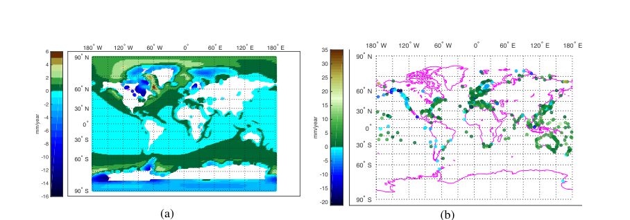
Demonstrates the challenges in modeling geospatial datasets.
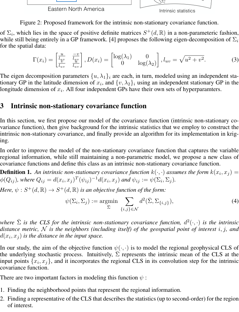
Visual representation of the modeling approach and its components.
Frequently Asked Questions
To compute the objective function ψ for the space of spatially smooth kernels ({Σ i } N i=1 ), we assume that ψ lies on the Riemannian manifold M of positive definite matrices S + (d, R). defined the empirical Riemannian mean.
Covariance functions are a key element in the regression of geospatial data (kriging). Finally, the CLS (ψ ij ) is used in Equation ( 2 ) for the GP regression model.
The standard kriging (GP) model tries to recover the underlying function, f , where y i ∼ f (x i ) + η, from n observed data points {(x, y)} n i=1 . The learned model is then used to compute the.
We used the empirical Riemannian mean rather than the arithmetic mean and, therefore, are free from fixing the bounds on the initial estimates of {Σ i } N i=1 . The high improvement is because TG has large variability in the regional.
Future work will explore the application and methods of our intrinsic covariance function to such geospatial datasets, with the larger goal of aiding in the assessment of future climate related risks.
This paper discusses a new way to model climate data, particularly sea level changes, by using a special mathematical function that adapts to different regions and conditions. This approach helps improve predictions about future climate impacts.